Probability sampling is not just a statistical nicety; it is the foundational step that determines whether your analysis has any claim to truth about the world beyond your dataset.
By thoughtfully choosing and implementing these methods, you move from making educated guesses to providing mathematically sound estimates with known uncertainty. And that is the true mark of a rigorous data scientist or statistician.
Table of Contents
As data scientists and statisticians, we live in a world of inference. We take a small, manageable piece of the world (called a sample: a small representative portion of the whole) and use it to make powerful claims about a much larger whole (called the population in statistics). But the bridge between that sample and the population is only as strong as the method we use to build it. That bridge is a probability sampling.
Forget black-box models and “garbage in, garbage out” for a moment. The most fundamental step in ensuring the statistical validity of your analysis starts right here, at the sampling stage. Today, we are diving deep into the why and how of probability sampling, the gold standard for any analysis that aims to be truly representative.
Probability Sampling
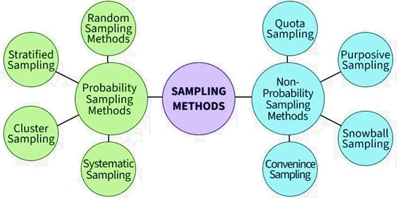
Probability Sampling is the procedure in which the sample is selected in such a way that every element of a population has a known or non-zero probability of being included in the sample. Simple random sampling, stratified Random Sampling, systematic sampling, and Cluster Sampling are some Probability sampling designs.
Why Probability Sampling is Non-Negotiable in Data Science
In a probability sampling design, every single member of the population has a known, non-zero chance of being selected. This one simple rule is what unlocks everything we hold dear in statistical inference:
- Unbiased Estimation: It allows us to calculate estimates (like the sample mean) that are unbiased with respect to the population parameter.
- Quantifiable Uncertainty: This is the big one. Knowing the probability of selection allows us to calculate the sampling error and construct confidence intervals. We can finally say, “We are 95% confident the true population mean lies within this range.” This is the bedrock of statistical confidence.
- Generalizability: The results from your sample can be legitimately generalized to the entire population you drew it.
Without probability sampling, you are left with non-probability sampling (like convenience sampling or voluntary response surveys), which is riddled with selection bias and offers no way to measure the error of your estimates.
The Core Methods of Probability Sampling: A Practical Guide
Let us break down the four workhorse techniques. Choosing the right one depends on your population structure, budget, and desired precision.
1. Simple Random Sampling (SRS)
- The purest form of probability sampling. Every possible subset of $n$ individuals has an equal chance of being the selected sample, and each possible sample with or without replacement has equal probability of being selected as a sample. It is like a lottery for your population.
- How: Assign every member a number and use a random number generator to select the sample.
- When to use: Ideal when your population is homogeneous (very similar). It’s simple to understand, but it can be inefficient or expensive if the population is large and spread out.
- Data Scientist’s Note: In Python, you can use
numpy.random.choice()orpandas.DataFrame.sample()to implement this easily on a frame.
2. Systematic Sampling
- In the sampling method, the sample is obtained by selecting every $k$-th element from a list of the population. You choose a random starting point between $1$ and $k$ and then select every $k$-th element after that. The $k$ is the sampling interval and stands for the integer nearest to $\frac{N}{n} = \frac{Population\, Size}{Sample\, Size}$.
- How: Calculate
k(the sampling interval) by dividing the population size (N) by your desired sample size (n). Start randomly and select every $k$-th item. - When to use: A simpler and more practical alternative to SRS when you have a complete sampling frame (e.g., a customer list, a phone book).
- Warning: Be cautious of hidden periodicities in the list that could introduce bias (e.g., sampling every 7th day might always land on a Tuesday).
3. Stratified Sampling
- Sometimes population units are not homogeneous according to certain characteristics. Dividing the population into distinct, homogeneous subgroups called strata (e.g., age groups, income brackets, product types), then performing a random sample within each stratum. The combined sample from each stratum is called a stratified random sample, and this whole procedure is called stratified random sampling.
- How: You can proportionally allocate the sample size to each stratum (e.g., if a stratum is 20% of the population, it gets 20% of the sample) or use optimal allocation to allocate more samples to strata with higher variability.
- When to use: Perfect when you want to ensure representation of key subgroups or when you know certain strata are more variable than others. It often provides greater statistical precision and reduces sampling error compared to SRS.
- Data Scientist’s Note: This is crucial for building training sets for machine learning models on imbalanced data (e.g., fraud detection) to ensure the model sees enough rare cases.
4. Cluster Sampling
- Dividing the population into naturally occurring, heterogeneous groups called clusters (e.g., cities, schools, factories). You then randomly select a subset of clusters and survey every individual within the chosen clusters.
- How: This is often done in multiple stages (multi-stage sampling), e.g., randomly select states, then cities within those states, then schools within those cities.
- When to use: Primarily for cost and logistics. It’s far cheaper to visit a few random clusters (e.g., five cities) than to sample individuals randomly spread across an entire country. The trade-off is that clusters are often similar internally, which can lead to higher sampling error compared to SRS.
Choosing the Right Sampling Design: A Quick Guide
| Method | Best For | Key Advantage | Key Consideration |
|---|---|---|---|
| Simple Random Simpling | Small, homogeneous populations | Conceptual simplicity, unbiased | Can be inefficient/logistically hard |
| Systematic Sampling | Having a complete list/frame | Easy to implement | Vulnerable to hidden patterns |
| Stratified Sampling | Populations with important subgroups | Increases precision, ensures subgroup representation | Requires prior knowledge to form strata |
| Cluster Sampling | Large, geographically dispersed populations | Major cost and logistical savings | Higher sampling error for same sample size |


