The quality of your video is too bad after uploading to Instagram Story? In this article, we will tell you why the video on Instagram Story is blurry and how to fix the Instagram Story video quality.

If you are a longtime Instagram user, you will realize the importance of video/ photo quality on Instagram. However, on social networks, you see a lot of people complaining about topics like this.
“My videos became of poor quality after uploading them to Instagram. There is no problem with the video. Why and how do I fix this problem? ”
Poor quality video on Instagram Stories can occur for many reasons, including Internet connection and app version. Whatever it is, the problem of poor-quality Instagram story videos is not difficult to solve. Follow the methods below and say no to blurred Instagram video stories. The methods below can be used to fix Instagram story video quality.
Ways to Fix Instagram Story Video Quality Problem
1. Check Internet connection
If your Internet connection is unstable, uploaded Instagram videos may be blurred because they have not been fully loaded. While you are uploading a video to Instagram with a poor Internet connection, Instagram will automatically reduce the quality of the video for upload. Try to connect your device with a stable WIFI adapter to mobile data.
2. Try different videos and images
Recovered your phone from a backup? Try a different video or photo. The clarity of photos and videos can change in the damaged backup.
3. Reset network settings
On an iPhone, to reset network settings, you have to go to Settings> General> Reset> Reset Network Settings. On an Android phone, you need to go to Settings> Backup and reset> Reset Network Settings.
4. Adjust camera settings
When your phone is unable to record high-quality video, here’s what you do to adjust your phone camera settings.
On Android:
Step 1: Open the default Camera app on your phone.
Step 2: Click the Settings icon, shaped like a gear.
Step 3: Adjust the image and video size to the highest quality.
On iPhone:
Step 1: Launch the iPhone Settings app on your phone.
Step 2: Find Camera.
Step 3: Adjust camera quality and turn on “Automatic DHR”.
5. The picture and video size is not the correct aspect ratio
Instagram limits the size and quality of the photos and videos you upload. If you’re uploading a video or photo that’s too large, Instagram compresses it so your video loads faster. One solution is not to use the phone’s camera. Use Instagram’s camera instead. No cuts and no quality loss.
6. Update the application
When you’re on an older version of Instagram, Instagram Story videos may appear worse. Update it so you can enjoy your new Instagram journey.
7. Adjust Instagram settings
Instagram burns your mobile data. To prevent you from misusing your data, Instagram gives you a setting to keep your mobile data usage to a minimum. This will dramatically decrease the quality of your Instagram feed. Here’s what you do to disable this setting.
Step 1: Launch Instagram and tap on your profile icon.
Step 2: Click on the three horizontal lines.
Step 3: Go to Settings> Accounts> Cellular Data Usage.
Step 4: Turn off Data Saver.
8. Use a photo/video editing app
Instagram has certain requirements for videos and photos. If the video you want to upload doesn’t meet the requirements, Instagram will automatically trim or compress it.
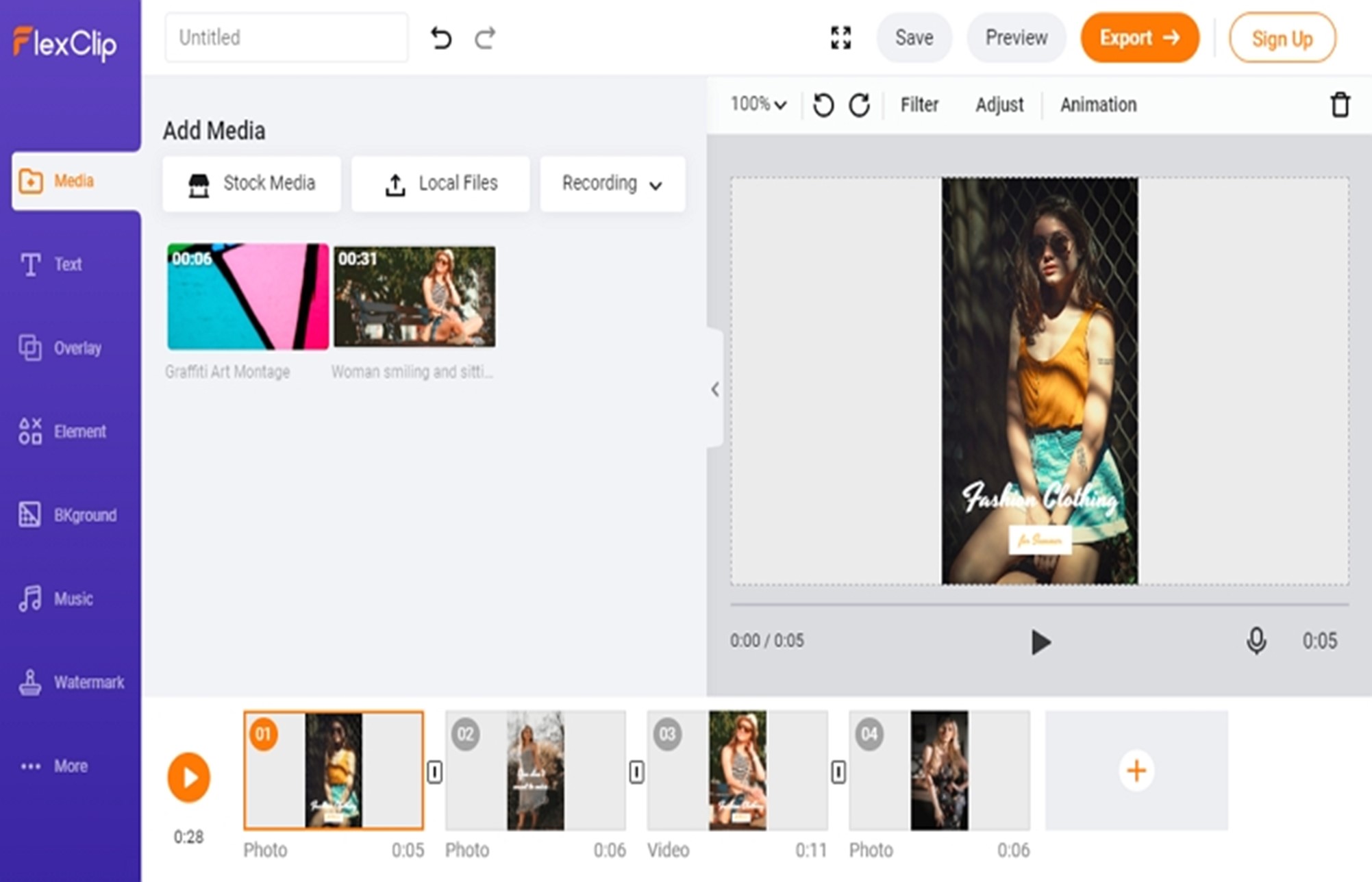
Lots of video editors like FlexClip help you crop and compress videos to fit the Instagram story format without losing video quality. In clicks, you can adjust the aspect ratio, video length, and video size.
Moreover, it also gives you other video editing tools for video upscaling, like transitions, filters, and video speed changers. Last but not least, FlexClip has a ton of media resources that you can apply, including video clips, photos, music, and even royalty-free pre-made video templates.
Conclude
With 8 solutions to poor-quality video processing on Instagram stories, you will no longer experience blurred Instagram video stories! Share this post if you found it helpful to fix Instagram story video quality.
Convert Documents to PDF, doPDF


