In SPSS (Statistical Packages for Social Sciences) split file option lets the user to splits the data into separate groups for analysis based on the values of one or more grouping variables. If user select multiple grouping variables, the cases are grouped by each variable within categories of the preceding variable on the groups based on list. Let us learn about the step-by-step procedure to Split Data file in SPSS.
How to Split Data File in SPSS
Suppose you want to take the separate mean of male and female (groups/ categories from gender variable) then one may use split file option.
First Open the data file you want to split.
Second, from the menu bar, click the Data Menu and then Split File Option (Data -> Split File)
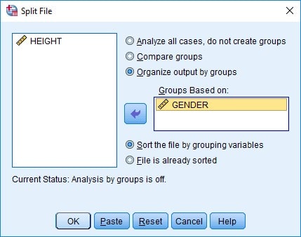
The following dialog box “Split File” will appears. Click on the radio button title “Organize output by Groups” after clicking the Grouping variable from left pan.
Select the Gender Varaible (or the grouping variable you want to split) in the dialog box at the left pan and clikc on the arrow at the “Groups based on” box.
Click the OK button. Now, subsequent analyses will reflect the split.
The data in data windows will be logical splitted. One can run requierd descriptive and inferential analsysi of the splitted data.
Split File Off
The most important point is to get back to ‘normal’ where the data are not split, go back to Data/Split Files… and select the option ‘Analyze All cases.’
Press OK. It will show SPLIT FILE OFF. Then you can get back output of data without splitting the files.
In this post, a discussion about diagnostics for a LeverageInfluential point and outlier will be made. In a regression analysis, certain observations may play a role in influencing the outcomes of the fitted model and its estimates. These observations may be classified as outliers, leverage, and influential points.
Table of Contents
Outlier Leverage Influential Point
The explanation of outlier leverage influential point is described as under:
Outliers: An outlier is an extreme observation that differs considerably from the other observations. An outlier may be due to the recording error and the model cannot explain them. However, outlier(s) may contain some important information. An outlier may be in $x$-space, $y$-space, or both.
Leverage: An unusual $x$ value is called a leverage point. The leverage point affects the model summary statistics (such as $R^2$, standard error, etc.), but has little impact on the estimates of the regression coefficients. A leverage point has an unusual predictor value and is different from the bulk of the observations.
Influence: An unusual $y$ value (and may be an extreme $x$ value), is called an influence point. An influence point has a noticeable impact on the estimated regression coefficients and may change the direction of the slope.
image taken from: https://www.cbsd.org/
Diagnostics for Outlier Leverage Influential Point
Outliers must be treated very carefully. Outliers may be detected by examining the
Normal Quantile Plots (departer from normality)
Residual Plots (magnitude of the residuals)
Scaled residuals (a potential outlier if magnitudes > 3)
Leverage Point
The diagonal elements of the “hat matrix” have an important role in detecting influential observations. $$h_{ii} = x’_i (X’X)^{-1}x_i,$$ where $X$ is matrix of regressors and $x’_i$ is the ith row of the $X$ matrix.
A large diagonal element is an indicator of influential observation as they are remote in $x$-space. Any observation exceeding the average size of the diagonal element of the hat matrix ($\overline{h} = \frac{p}{n}=2h$) is considered as a leverage point, where $p$ is the number of parameters in the model. It is also useful to observe the studentized residuals in conjunction with $h_{ii}$ (that is, look for large hat diagonal and large residual values).
Note that not all of the leverage points are influential unless they have large residuals. Therefore, observations having large $h_{ii}$ values and large residuals are likely to be R.
Influential Points
Cook’s Distance: The Cook’s Distance is the Deletion Diagnostic that is used to measure the influence of the $i$th observation by removing it from the regression analysis. It is based on all $n$ points, $\hat{\beta}, and the estimates based on the deletion of the $i$th point, $\hat{\beta}_{(i)}$.
DFBETAS is another Deletion Diagnostic used to measure how the change in each of the $\hat{\beta}j$ is due to influential observation. A large value of DFBETAS indicates that the $i$th observation is considerably an influential observation on the $j$th regression coefficient. If $|DFBETAS{j, i} > \frac{2}{\sqrt{n}}$ then the $i$th observation warrants further examination.
DFFITS is another deletion diagnostic measure used to measure the deletion influence of the $i$th observation on the predicted or fitted values. DFFITS is the number of standard deviations that the fitted values change if ith observations are removed. If $|DFFITS_i|>\frac{2}{\sqrt{\frac{p}{n}}}$ then the $i$th observation warrants further examination.
Note that the case deletion diagnostics do not provide any information about the overall prediction of the estimation. However, the performance of the model can be measured by using the Generalized Variance (GV) and Covariance Ratio.
In summary, the Outliers, Leverage Points, and Influential Observations are certain data points (observations) that deviate (distant) from the expected patterns. On the other hand, the outliers are extreme values that lie far away from the other data points, while leverage points exert a strong influence on the regression models.
The Online sampling Quiz with Answers is about the Basics of Sampling and Sampling Distributions. It will help you understand the basic concepts of sampling methods and distributions. This Sampling Quiz will help the students prepare for different exams related to education or jobs. Most of the MCQs on this page cover MCQ Sampling Quiz with Answers, Probability Sampling and Non-Probability Sampling, Mean and Standard Deviation of Sample, Sample size, Sampling error, Sample bias, Sample Selection, etc.
Multiple Choice Questions about Sampling and Sampling Distributions
Sampling Quiz With Answers
A procedure in which the number of elements in a stratum is not proportional to the number of elements in populations is classified as
Cluster sampling, stratified sampling, and systematic sampling are types of
The listing of elements in a population with identifiable numbers is classified as
There are 50 students in a class. A data analyst wants to know if a majority of students like the instructor. They decided to survey the 15 students who earned an A in the class because these students were paying attention to the instructor. Which of the following statements best describes this sample?
When Hartley-Ross proposed the unbiased ratio estimator?
Which of the following sampling methods is the best way to select a group of people for a study if you are interested in making statements about the larger population?
The auxiliary variable is also called
The average of cluster means is the unbiased estimator of a population mean when
In cluster sampling, elements of selected clusters are classified as
Sampling in qualitative research is similar to which type of sampling in quantitative research?
Which of the following would usually require the largest sample size because of its efficiency?
All of the following are true about cluster sampling except
The human resources department at company XYZ has 42 workers in int. To find out some information about the group as a whole, we want to take a sample of 7 of those workers to interview. If we have an ordered list of workers numbered 1 through 42, and we start at worker number 3, which worker would be included in our sample?
If a statistician randomly samples 50 observations in each population category then his sample will be ———-.
In which of the following non-random sampling techniques does the researcher ask the research participants to identify other potential research participants?
In systematic sampling, when $N=18$ with $n=3$ what will be the value of $k$?
In systematic sampling, the value of $k$ is classified as
If we took the 500 people attending a school in a city, divided them by gender, and then took a random sample of males and a random sampling of females, the variable on which we divide the population is called the
In a double sampling plan, if the number of defects is in between the two numbers C1 and C2 then
Which ONE of the following is the main problem with using non-probability sampling techniques?